Tired of the same old formatting in Excel and want to break the monotony? You can color alternate rows in a spreadsheet. That’s one regular row, then a colored row.
You know that will look good on the Excel sheet.
However, apart from breaking the monotonous data formation, highlighting alternate rows can be helpful when sorting specific data from the worksheet.
That could be sorting the product list… Sorting employee details and/or other geeky excel works.
To highlight every second row in MS Excel, you can simply use the table formatting, try conditional formatting, or use different excel functions.
This article will go through every possible method to highlight every other row quickly. So, could you bare with me till the end?
Check out our separate post on how to Sort by Date in Excel
How to Highlight Every Other Row in MS Excel
The fastest way to shade every other row in Excel is manually select the rows and highlight them with preferable color. Just hold the Ctrl key on your keyboard and click on the rows you want to highlight. When you select all the rows, click on the fill color button in the Home tab.
This method only works when the Excel rows are limited. If you’re managing a large data set, using this method can cost you a lot of time.
Try the following techniques if that’s the case.
Read more on how to Excel Documents Open in Notepad on Windows 11
Here are the methods to highlight every second row in Microsoft Excel:
1. Shade Alternate Rows using Table Styles
When you’re sorting a large number of rows from a spreadsheet, shading every other row can be really difficult with just using a mouse and keyboard. You can try table styles to shade every second row in excel.
Here are the steps to shade every other row in Excel using table styles:
- Select the range of data you want to highlight alternatively.
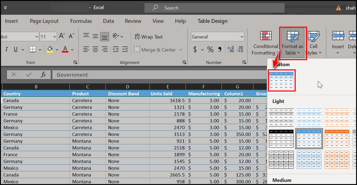
- Click on the Format as Table button in the Styles group.
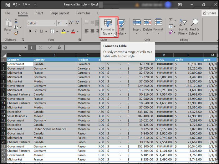
- Choose the table style that you prefer most. A dialog Format As Table will pop up to verify the range of selected rows.
- Click OK if the range is correct.
Note: You can change the table style, even the color that you chose. Click on the format as table button again and apply the table formatting you prefer.
If the rows are not highlighted even after formatting the table, select the table and go to the Table Design tab. Make sure that the Banded Rows option is marked in the Table Style Options group.
Read more on how to Copy & Paste Objects in Excel
2. Create Custom Table Format to Highlight Every Other nth Row
Let’s say you don’t need to shade every second row in Excel. Instead, it would help if you colored every fourth row/ fifth row on your spreadsheet.
I can assure you that’s possible. You need to be a little bit patient and follow my instructions.
Here’s the procedure to create a custom table in Excel that can color every other nth row:
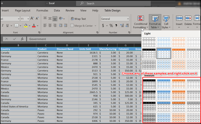
- Open the Excel sheet and click on Format as tables.
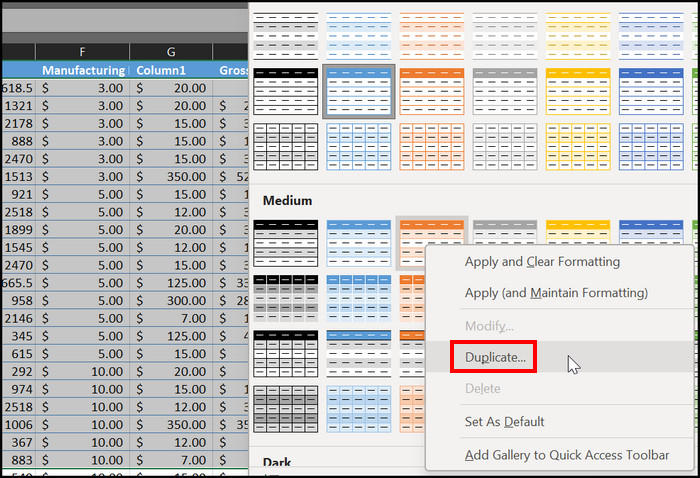
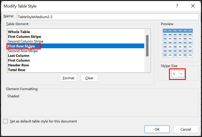
- Right-click on any of the table styles and select duplicate. This will open a dialog box named Modify Table Style.
- Click on the First Row Stripe option from the list and set the Stripe Size as 1.
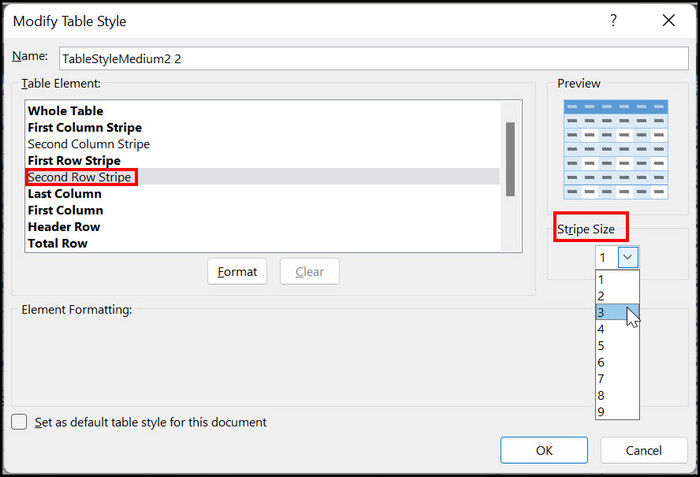
- Select the Second Row Stripe option and set the number of rows you want to cut from the Stripe Size menu. Suppose you’re highlighting every fourth row. So, select 3 in the strip size dropdown menu.
- Set a name for the table format you just created and click Ok.
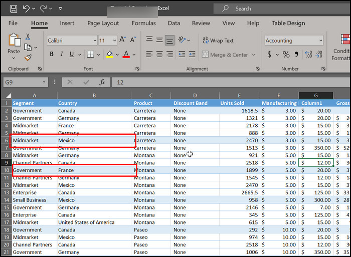
After that, select the range of data you want to highlight and click on Format as tables in the Home tab. You’ll notice a custom table style is available there. Click on it, and you’ll notice every fourth row is highlighted.
Note: If you want to color every 5th row, select the second-row strip option and set the strip size dropdown menu as 4.
Follow our guide on how to Mail Merge in Outlook with Excel & Word.
Highlight Alternate Rows Using Conditional Formatting
Using conditional formatting to color every second row in Excel is also time-efficient. There’s no need to skip this part if you’re not good with formatting. I’ll explain conditional formatting so easily that you’ll be able to color the rows after reading this tutorial.
Here are the steps to color alternate rows using conditional formatting:
- Launch MS Excel on your device and select the range of cells you want to shade alternatively.
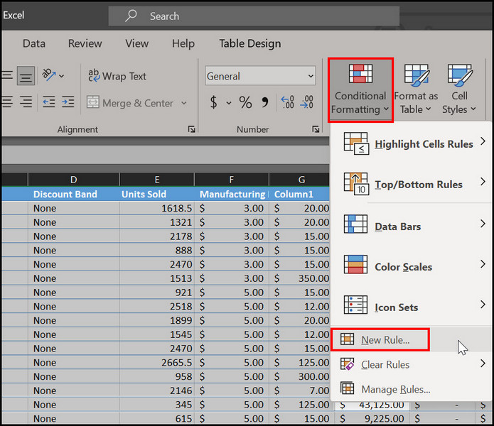
- Click on Conditional formatting on the Home tab.
- Select New rule from the dropdown menu.
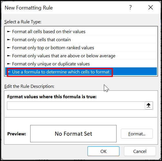
- Choose the Use a formula to determine which cells to format option when the New formatting rule window appears.
- Click on the Format Values when this formula is true box and type in this formula =MOD(ROW(),2).
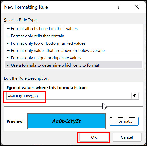
- Click on Format to pick an appropriate formatting style.
Note: Make sure you use a light shade to highlight the rows to make the rows readable.
Apply Color to Every Other Row in Excel Mac
If you’re using Excel on macOS and want to apply shade to every other row, this guide might help you. Excel in Mac is not so much different from the Windows version. You’ll find similarities while coloring alternate rows.
Here are the steps to apply color to alternate rows in Excel Mac:
- Select the range of rows that you want to highlight.
- Move to the Insert tab > select Table.
- Tick on My table has headers; if your data has headers, then click OK.
- Select the table style that you prefer from the Table tab.

- Select Convert to Range on the Table tab in case you want to remove the sort and filter arrows.
- Click on Yes to complete the shading.
See? That’s not even a little complicated as you thought beforehand. You can shade the entire spreadsheet in this manner.
Here’s a complete guide on how to Copy Values Without Formulas on Excel
Excel Highlight Every Other Row if Not Blank
By default, Excel highlights every cell even if the cells are blank. Sometimes, it can create destruction while sorting data.
You can solve those irregularities by using the conditional formatting rule. But, unlike the previous conditional formatting, you need to be a bit tricky this time. The rule you’ll use is called Format only cells that contain.
Let’s get into how you skip highlighting the blank rows.
Here’s the procedure to apply color to every other row if not blank:
- Select the dataset you want to highlight and move to Home > Conditional Formatting > New Rule.
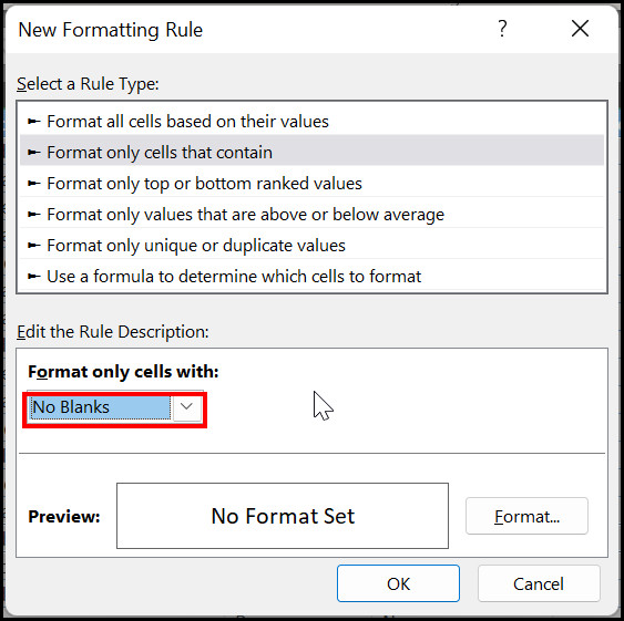
- Select Format only cells that contain from the New formatting rule window.
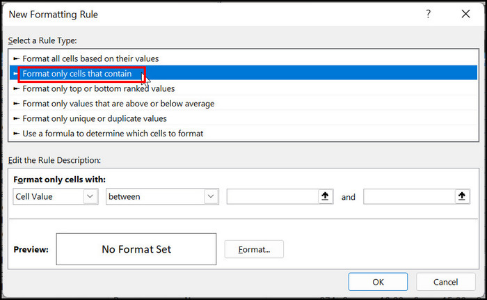
- Choose No Blanks in the Format only cells with the menu.
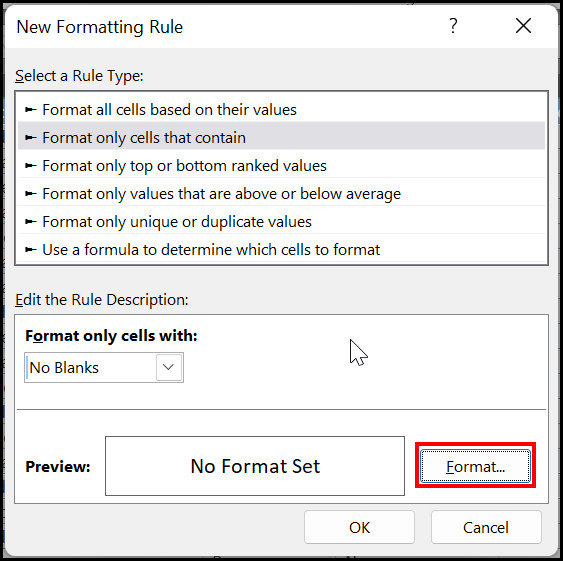
- Click on Format from the bottom right; the Format cells window will appear.
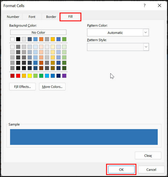
- Go to the Fill tab > select a preferable color and click OK. After that, get back to the New formatting rule window.
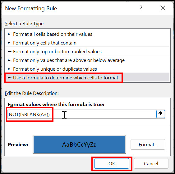
- Select the option Use a formula to determine which cells to format.
- Type this formula in the empty box below; NOT(ISBLANK(A3)).
- Click on Ok to finish the process.
You’ll notice every cell is highlighted except the empty cells on your worksheet. This way, you can eliminate the cells that are not necessary or even fill them with data.
These are the proven methods of highlighting every other row in Microsoft Excel. If you have any other queries related to this topic, feel free to read the subsequent sections.
Frequently Asked Questions
How do I highlight every other row in Excel 2020?
Select your worksheet data > Press Alt + O + D > In the conditional formatting menu, click on Use a Formula to determine which cells to format option > Enter this formula in the emply box; =MOD(ROW(),2) > click ok.
How do I shade alternate rows in Excel without a table?
Hold the Ctrl key on your keyboard > select the rows you want to be colored > Click on the Fill color icon in the home tab > choose the shade you want to use.
How to highlight every odd/even row in Excel?
Create a new custom table in Excel > Select the first row stripe from the table element > Set the stripe size to (2,4,6 for highlighting even-numbered rows) (1,3,5 for highlighting odd-numbered rows).
Wrapping Up
Applying colors on Excel rows is fun. And I can assure you, after reading this article, it’ll be even more satisfying to color different shades on an Excel sheet. Not to mention, it’ll help you sort data.
Here, I used multiple highlight techniques, and every one of them works perfectly. Don’t forget to comment on which of these methods you liked the most.