Sometimes, while managing a large amount of data, you’ll notice there are exact values replicated in the spreadsheet. You might spot the duplicated data in different cells, rows, or columns.
That makes your spreadsheet clumsy and difficult to understand.
To make your excel sheet more understandable and accurate, you can find out and emphasize the repeated values.
This article will help you with the methods to quickly locate and mark duplicate values in Microsoft Excel 2013, 2016, 2019, and Excel 365.
So, without wasting any more time, let’s dive deep into Microsoft Excel.
Check out our separate post on Fix Microsoft Excel Freezing or Slow
How to Highlight Duplicates in Microsoft Excel
Select the data range you want to check for duplicate values. Go to the Home tab of your Excel Sheet. In the Style section, click on conditional formatting > Highlight Cells Rules > Duplicate Values. Choose your preferred color and select Ok. Alternatively, press Alt+H+L+H+D to highlight them.
That’s one of the easiest methods you can implement to highlight duplicate values. However, there are multiple techniques to find identical excel values. Continue reading to find them.
Here are the methods to Highlite duplicate Excel data:
How to Highlight Duplicate Cells in Microsoft Excel
If you want to highlight the non-unique cells in the spreadsheet, following these steps might help you. Mostly, conditional formatting is the key to highlighting those replicate data.
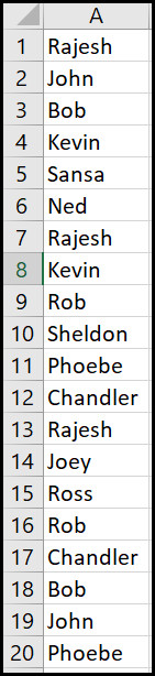
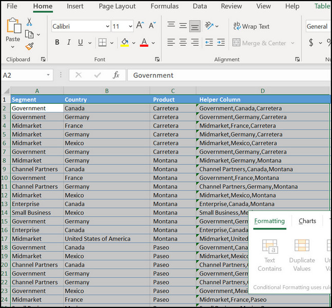
I’ve added a sample spreadsheet photo with duplicate values for your better understanding. Open the excel sheet on your computer and practice as I explain.
Here are the steps to emphasize duplicate cells in Excel:
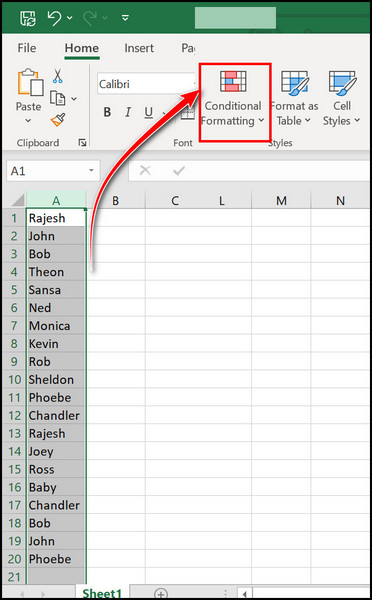
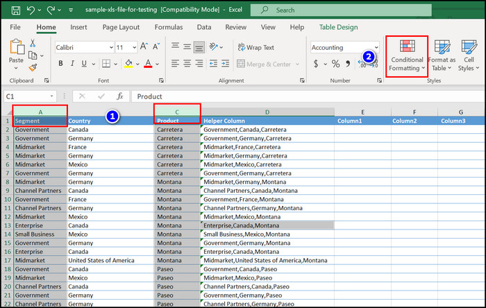
- Select the column that has a duplicate data range.
- Click on Conditional Formatting in the Home tab.
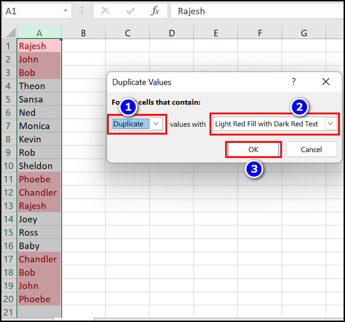
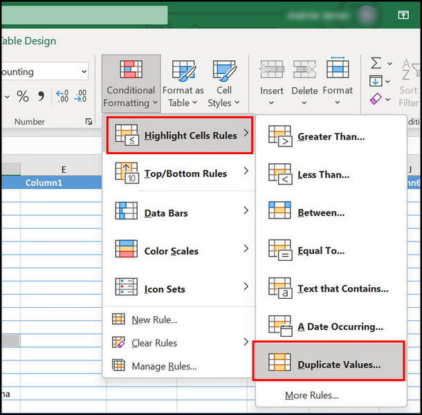
- Navigate to Highlight Cells Rules > Duplicate Values. You’ll notice two drop-down menus in the forthcoming window.
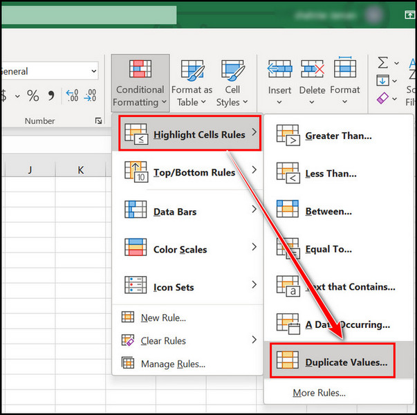
- Select Duplicate in the first one and select your preferred color in the second. E.g., Light red fill with darker red text.
- Click Ok to confirm the highlight.
You’re all set. You’ll notice the duplicate data marked as red in your excel sheet. Also, you can find duplicate rows in the spreadsheet and highlight them. Check out the following method if you want the rows highlighted.
Here’s a complete guide on how to Copy Values Without Formulas on Excel
Find and Highlight Duplicate Rows in MS Excel
When all the available data you have on the spreadsheet is saved more than once, you might want to use this technique. Duplicate rows will show up as highlighted after you follow this guide.
Most users get afraid of using the excel formula. But, I can assure you if you follow my instructions, identifying duplicate rows won’t be an issue.
Here are the steps to highlight duplicate rows using a simple formula:
- Open an Excel sheet on your computer.
- Select the rows in which you want to find duplicated data.
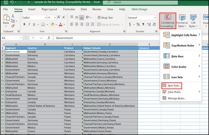
- Click on Conditional formatting from the Style section.
- Select New rule from the list. A new window will pop up.
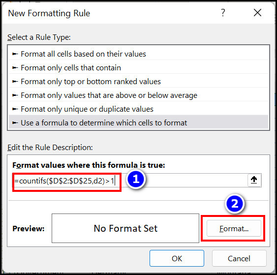
- Click on Use a formula to determine which cells to format.
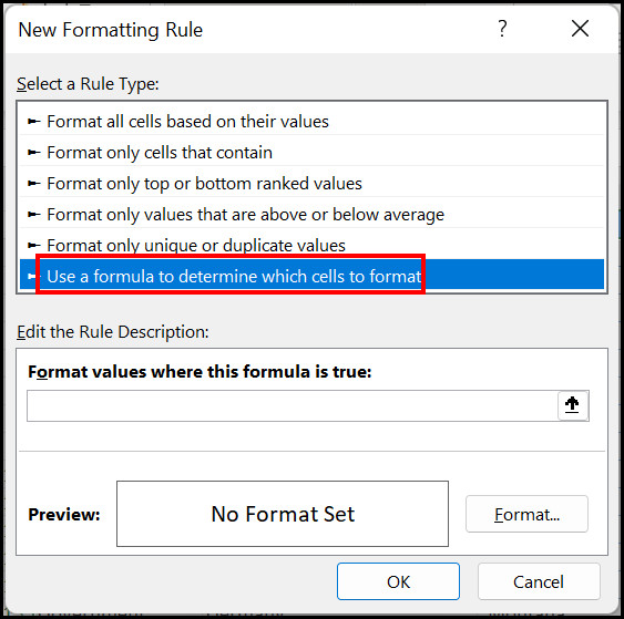
- Edit the rule description and type this formula; =countifs($D$2:$D$25,d2)>1
- Click on Format from the bottom right corner.
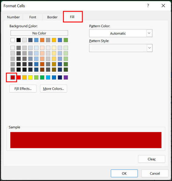
- Navigate to the Fill tab and select a color. For instance, I selected red.
Note: The formula I wrote here won’t match your spreadsheet. Make sure you change the cell and row number according to your data.
Now, if you want to highlight duplicate data from multiple columns, check out the further instructions.
But before that, go through our epic guide on how to Lock and Unlock Cells in Excel
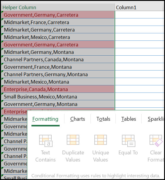
How to Highlight Duplicates from Multiple Columns
Spotlighting multiple column data in your excel sheet is quite similar to the process you’ve read till now.
Just follow the instructions I will share next, and you will be able to highlight Highlight Duplicates in Multiple Ranges.
Here’s the process to highlight duplicates in different excel ranges:
- Select all the columns from where you want to rule out the non-unique data.
- Press Ctrl + left click on your mouse if the columns aren’t adjacent.
- Click on Conditional formatting from the dashboard.
- Select Highlight Cells Rules > Duplicate Values.
- Choose your preferred color from the next window and click Ok.
That will mark the replicated values from your spreadsheet. And if you want to delete the duplicate data, check out the following section.
Check out our separate post on How to Install Macro in Excel
How to Remove Duplicate Values from Excel Sheets
Deleting the duplicate values from a spreadsheet is one of the easiest workloads, if not the easiest. Just work along with the techniques that I’m going to share, and you’ll be fine.
But before you delete the duplicate data, I would recommend you keep a copy of the original data, just in case.
Here are the steps to delete duplicate values from MS Excel:
- Open the Excel sheet on your computer.
- Select the column(s) that has a duplicate value.
- Go to the Data tab and click on the Remove Duplicates sign from the dashboard. A new window will pop up.
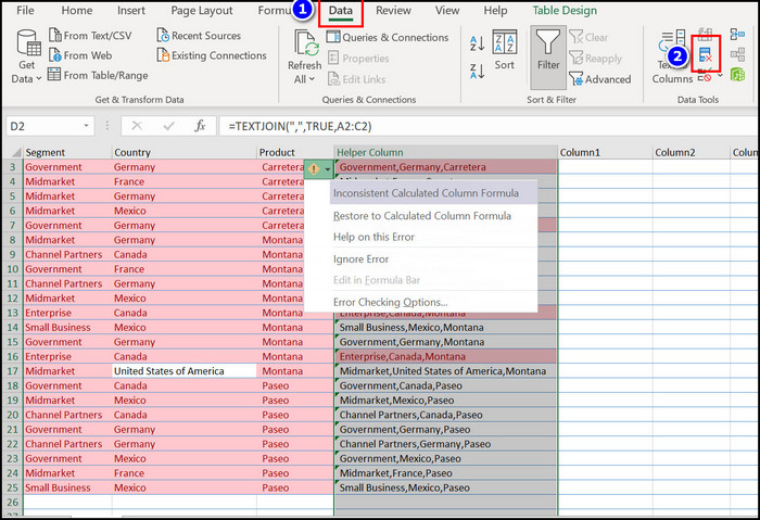
- Select the columns you want to remove duplicate data from.
- Click ok to finalize the process.
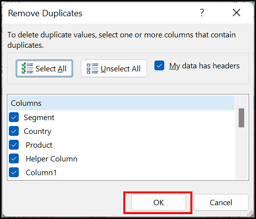
Note: If you’ve marked the column headers by mistake, tick on the My data has header option in the Remove Duplicates window. Your header column won’t be deleted then.
Now that you know how to find non-unique data in MS Excel and how to delete them, your data will be much more accurate from now on.
However, check out further sections if you have any questions regarding Excel duplicate data.
Also, check out our separate post on 12 ways to Fix Microsoft Teams Keeps Freezing My Computer
Frequently Asked Questions
How to highlight duplicates in two columns in Excel?
Select the individual columns that have duplicate data > click on conditional formatting > Highlight Cells Rules > Duplicate Values.
How to highlight duplicates in excel?
Open Excel > Click on the column you want to highlight the values > Conditional formatting > Highlight cells rule > Duplicate value > Click ok. Or, Open Excel > click on the column > Press and hold Alt + press H + L + H + D (one by one).
How to Delete Duplicates in MS Excel?
Select the individual columns that have duplicate data > Move to the Data tab > click on the remove duplicate sign > click ok. Or, press and hold Alt + A + M while selecting the highlighted column.
Conclusion
If you’ve read and followed the instructions I provided throughout the article, I can assure you will be able to mark the duplicates on your own.
However, make sure you use the latest versions of Microsoft Office (Office 2013-2019). Comment down which method helped you to identify the duplicate values in Excel. Share this article with your friends.