Microsoft Excel is vastly used worldwide for its graphing tools, pivot tables, calculation, and computation capabilities.
Nowadays, graphs and charts are needed for offices, schools, and colleges. With the help of those charts, we can easily understand the displayed data.
However, sometimes in a bar graph chart, some data level bars can be so massive that other bars look so tiny compared to the big ones. In those cases, inserting a break among the big bars can make your chart more attractive and understandable.
I researched and found that this breaking chart bar process is very complicated. So I formulate a simple yet functioning method with which you can easily break a bar chart axis in MS Excel.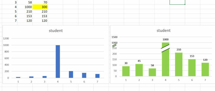
Don’t skip and read till the end to learn about a fantastic way to insert a break in Excel.
Let’s start!
What is an Axis Break in a Bar Graph on MS Excel?
An axis break means the discontinuity of values in an axis on MS Excel. Depending on your Excel modification, this value disruption can appear on the X or Y axis. This axis break is also known as the bar chart axis break, scale break, or graph break.
The Axis break looks like a wavy or straight line, with a blank space between these lines. In a chart, when other value bars are relatively small compared with the big bar, this axis break option comes into play.
With the help of this axis break option, you can make your big graph bars more readable and noticeable. Also, the total charts look very compact and eye-cache when you apply this axis bar break feature on Microsoft Excel.
Follow through the next heading, where I demonstrate how you can break a bar chart axis in Excel with some simple steps.
Read more on how to Excel Documents Open in Notepad on Windows 11.
How to Break a Bar Chart Axis in Microsoft Excel
After researching a lot, I found that breaking a bar chart axis or adding a break in the chart on MS Excel is difficult. Don’t worry; keeping all that in mind, I developed a super easy and working method with which you can add a break in your chart axis bar.
Here are the steps to break a bar chart axis in Microsoft Excel:
1. Make a Plan on How you Want to Break the Bar Chart in Excel
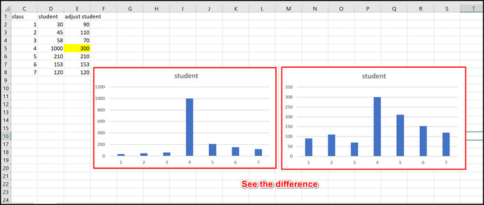
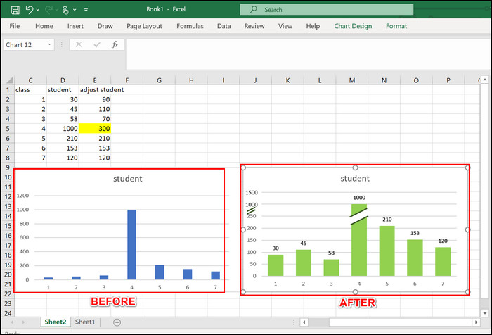
Useful planning is essential before breaking the bar chart axis in Microsoft Excel. For this article, I constructed a chart of a school with classes 1 to 7. But in class 4, the student limit hits the mark of 1000.
| Class | Student | Adjust Student |
|---|---|---|
| 1 | 30 | 30 |
| 2 | 45 | 45 |
| 3 | 58 | 58 |
| 4 | 1000 | 300 |
| 5 | 210 | 210 |
| 6 | 153 | 153 |
| 7 | 120 | 120 |
So when I make the table from the specific chart; the table doesn’t look good. So I changed the limit for class 4 and made 300 students in it. Then constructed the table again, and now it looks nice and clear.
After building a nice eye cache table, you can change its limit to normal and insert a bar chart break into that graph. You can see the highest limit for the student is 1000, and the second highest limit is 210, so I am going to break my axis between 210 and 1000 to shorten my table.
Here are the steps to make a plan on how to axis break in MS Excel:
- Open the MS Excel application.
- Make your desired chart and construct a table with them.
- Copy the Table and paste it beside the first table.
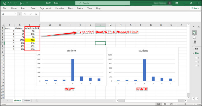
- Expand the chart with your Planned number.
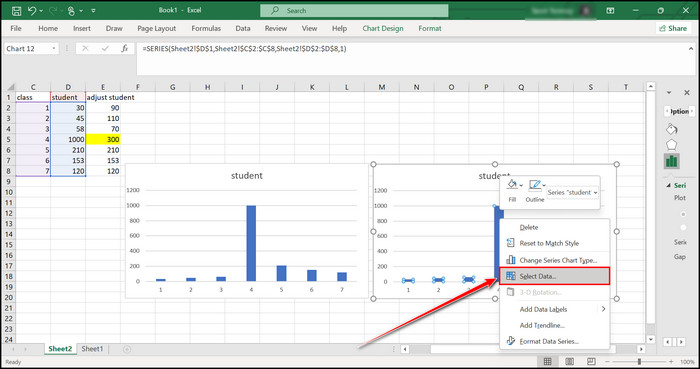
- Right-click on the Big Bar from the right-sided table and choose the Select data option.
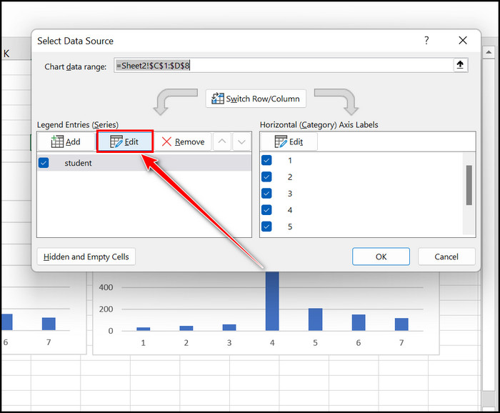
- Click on the Edit option and clear the Series Values box.
- Copy the expanded portion of the chart and paste them into the Series Values box.
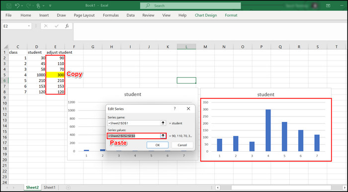
- Hit the OK button.
You can see that the right-sided table shows all the values from the expanded chart and looks very good.
Here’s a complete guide on how to Lock and Unlock Cells in Excel.
2. Include Data Label on your Bar Chart Axis in MS Excel
When your new table is ready, you can modify it and include the data label on your bar chart axis to make it more evident and noticeable.
Here are the steps to include the data label on your bar chart axis in MS Excel:
- Right-click on the Big Bar from the new table and select the Format Data Series option.
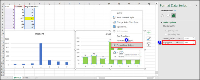
- Move to the Gap Width section and Lower it to make your table clearer.
- Right-click on the Big Bar again and select the Add Data Labels option.
- Click on the Value Data and move to the Level Options.
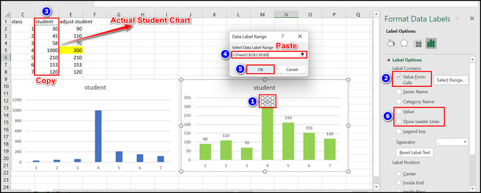
- Check the Value From Cells box.
- Copy the Actual Student Chart and paste it to the Select Data Label Range box.
- Uncheck the Value and Show Leader Lines checkbox, and your actual student chart is now implemented on the table.
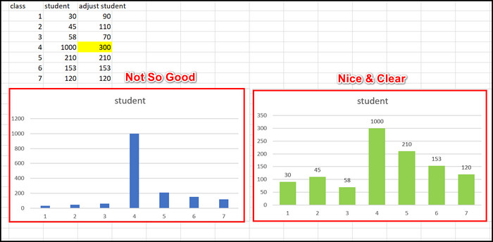
From the new table, you can see the real student count from the chart. Now it’s time to create a break into the axis of MS Excel; let’s follow the next heading to learn that.
3. Create a Broken Axis Shape for the Bar in Excel
The time has come to create a broken axis shape for the bar in Microsoft Excel. Move to the Insert section and Choose a rectangular shape; modify this to create a broken Axis in MS Excel.
Here are the steps to create a broken Axis shape for the bar in Excel:
- Navigate to the Insert menu and select a Rectangular shape.
- Draw it in the Excel sheet.
- Select the Line Shape from the Insert menu and overlap it on the Upper Portion of the Rectangular shape.
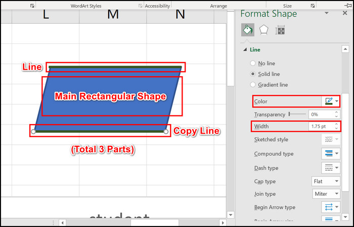
- Right-click on this Line and select the Format Shape option.
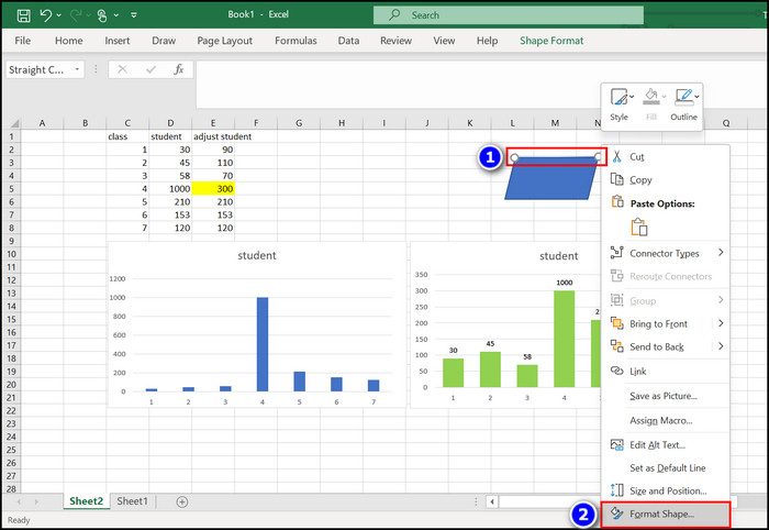
- Increase the Width of this Line and Change its Color according to your need.
- Press the CTRL+C button to copy this Line and type CTRL+V keys to Paste this line; now place the Pasted Line in the Lower portion of this line.
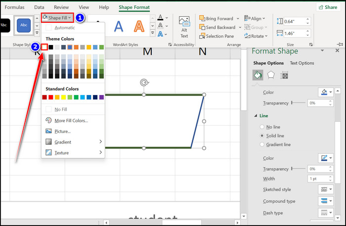
- Move to the Shape Format menu and select the Shape Fill to White color.
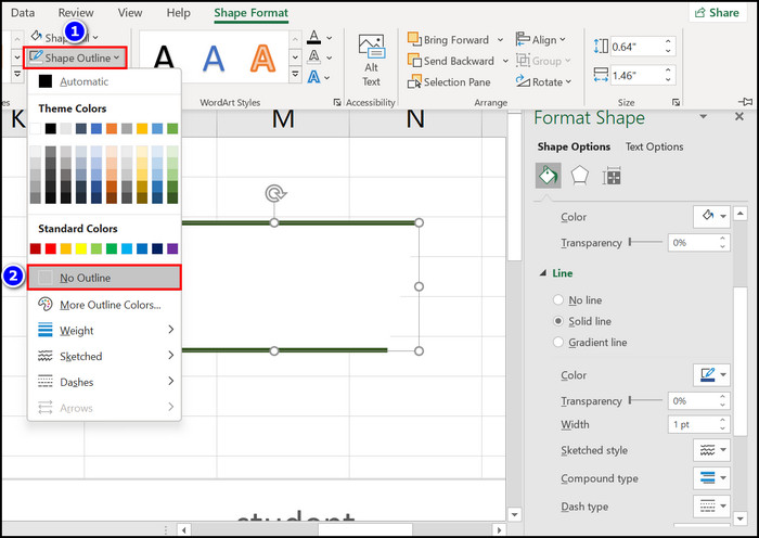
- Select the No Outline box from the Shape Outline option.
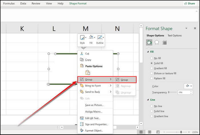
- Press the CTRL key and click on the Three Parts of this Shape to select all of them.
- Right-click and choose the Group option.
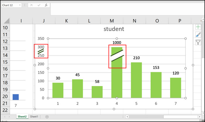
- Rotate the shape and Place it into the Big Bar.
- Copy the shape, Paste it using the CTRL+C and CTRL+V keys, and place the pasted shape into the Y-Axis.
Your bar chart axis is broken, but some modification still remains, so track down the following heading.
Here’s a complete guide on how to Copy Values Without Formulas on Excel.
4. Make a Similar Text Box to Overwrite the Y-Axis in MS Excel
To complete the axis bar break process, you must overwrite the Y-axis value data. Just select a rectangular shape and cover the extra Y axis with that. Create relevant values and place them on the blank Y axis.
Here are the steps to make a similar text box to overwrite the Y axis in MS Excel:
- Navigate to the Insert menu, select a Rectangular shape, and place it on the Extra Value Data.
- Move to the Shape Format menu.
- Choose the White option from the Shape Fill section.
- Select the No Outline checkbox from the Shape Outline option, and you will notice that the extra value data has vanished.
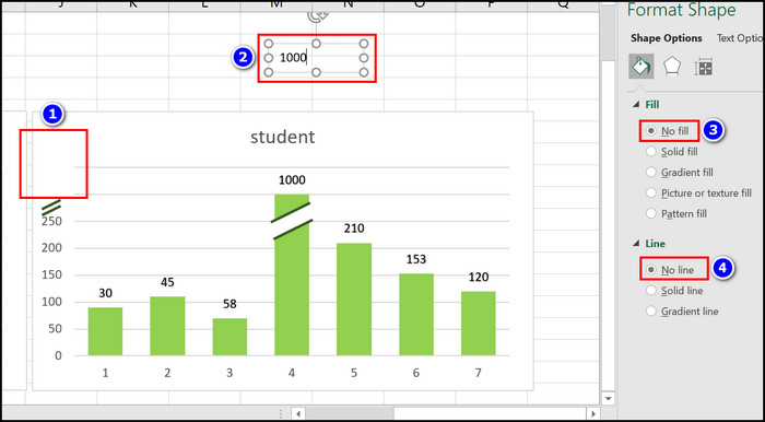
- Move to the Insert section and choose the Text Box option.
- Type your required Number, select the No Fill and No Line checkbox from the Fill & Line option.
- Match the number format with your excel sheet; for me, the format was Calibri 9.
- Place your number into the Y-Axis parallel with the line.
Congratulations, you completed the axis bar-breaking process.
Check out our separate post on how to Install Macro in Excel.
FAQs
How do you put a Line break in MS Excel?
To put a line break in Microsoft Excel, you must press the ALT+ENTER keys.
What is the Excel code for a line break?
The MS Excel code for a line break is 10 for Windows and 13 for the Mac OS.
How do I insert a line break in MS Excel for Mac?
If you want to insert a line break in MS excel on Mac, you must press the Control+Option+Enter buttons.
What does Ctrl+E do in MS Excel?
When you press the Ctrl+E keys on MS Excel, it will open the Flash Fill Feature.
What does Ctrl+M do in Microsoft Excel?
Pressing the Ctrl+M keys in MS Excel will store the current MS Excel calculator value.
What does Ctrl+Q do in MS Excel?
If you want to remove the entire format from a selected paragraph, you can press the Ctrl+Q button.
What does Ctrl+F do in Microsoft Excel?
When you press the Ctrl+F keys on MS Excel, it will open up the Find & Replace window.
What is a line breaker in MS Excel?
With the help of the Line breaker feature on MS Excel, you can break a line from a selected Excel sheet.
Afterthought
MS Excel is an excellent application with the help of which you can easily create your desired graph, chart, and table. But breaking the bar chart axis from MS Excel can be a challenging task.
However, upon my research, I found a straightforward and functioning method to break the axis bar in Microsoft Excel.
In this article, I demonstrate that process in detail, so read carefully and follow the procedure to complete the axis-breaking task successfully.
Do you have any queries related to this content? Let me know in the comment box.