There are about 16000 columns and more than a million rows in MS excel. Even if one-fourth of these cells are filled with data, and you have to work with those… I can feel you.
The problem with comparing hundreds of rows and columns is that the headers in the top row disappear when you scroll down to view lower entries.
You can solve this problem by freezing the rows and columns in Excel. In this article, I’ll explain how you can freeze panes to lock rows and columns in Microsoft Excel with straightforward steps. You can apply these tips to Excel 2013, Excel 2016, 2019, and every available excel version.
Also, this method works with Google Sheets, OpenOffice, and LibreOffice.
Keep reading till the end to find out.
How to Freeze Panes to Lock Rows and Columns in MS Excel
Freezing panes can be really useful to lock the header row and column in MS Excel. When you’re collaborating on multiple data sets in one spreadsheet, freezing the top pane can help you compare data with the existing ones.
Check out the following process to freeze rows and columns in MS Excel.
Here are the steps to freeze panes in Microsoft Excel:
How to Freeze Rows in Excel
In case you need to freeze only the rows of the excel sheet, this process will definitely help you. Read further down to lock multiple rows from the top in your spreadsheet.
Here are the steps to freeze rows in MS Excel:
Freeze the Top Excel Row(Header)
- Open the Excel sheet you want to modify.
- Go to the View tab.
- Click on Freeze pane > Freeze Top Row.
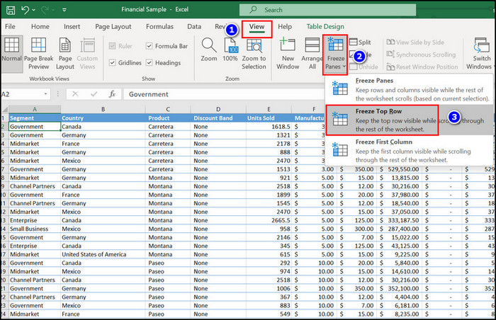
Note: A slightly dark border will appear if you lock a row successfully. The header row will always show when you freeze rows in Microsoft Excel.
Here’s a complete guide on how to Copy Values Without Formulas on Excel.
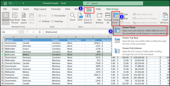
Lock Multiple Rows on Top
- Open Microsoft Excel on your computer.
- Select the row below the last row you want to freeze. For instance, click on the sixth if you want to lock the first five rows.
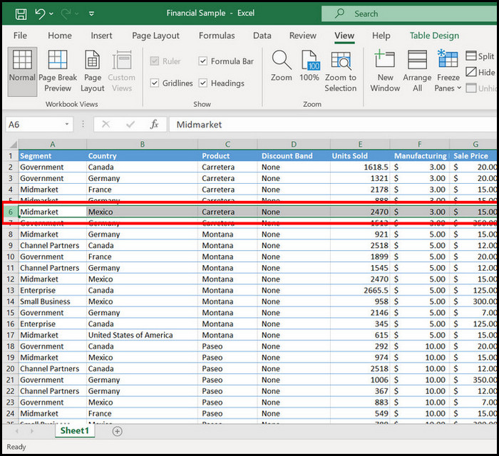
- Go to the view tab and click on the Freeze pane.
- Select the Freeze pane again when the drop-down menu appears.
Note: Make sure you select the row immediately below the rows you want to lock. If you want to freeze the top four rows, click on fifth. If you want the top ten, click on eleventh.
But before that, go through our epic guide on how to Lock and Unlock Cells in Excel.
How to Freeze Columns in Excel
Freezing columns in Microsoft Excel takes the same process as locking the rows. You just need to select the desired column and change its appearance from the view tab.
Here are the steps to freeze columns in Microsoft Spreadsheet:
Lock the First Column
- Open the Excel sheet on your computer.
- Click on the View tab.
- Select Freeze panes > Freeze first Column.
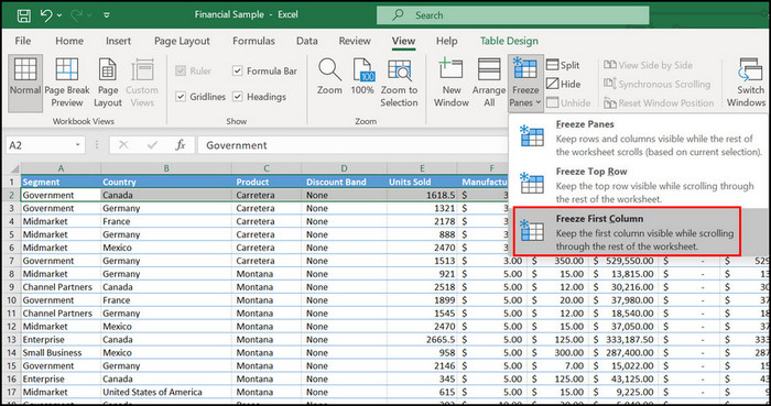
Note: A darker grey border means the column you selected is frozen.
Check out our separate post on how to Install Macro in Excel.
Freeze Multiple Columns in Excel
- Open Microsoft Excel on your computer.
- Select the column right side of the last column you want to freeze. For instance, click on the fourth if you’re going to lock the first three columns.
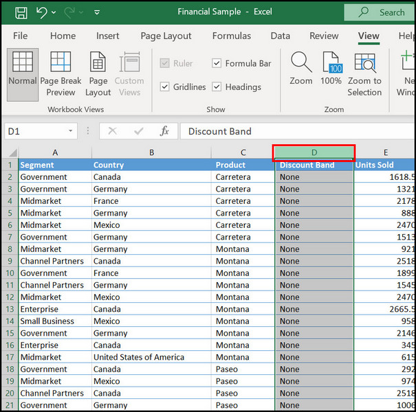
- Go to the view tab and click on the Freeze pane.
- Select the Freeze pane again when the drop-down menu appears.
Quick Tips: If you want to lock columns A-C, click on column D. Then go to the view tab > Freeze panes > Freeze Panes.
Also, check out our separate post on 12 ways to Fix Microsoft Teams Keeps Freezing My Computer.
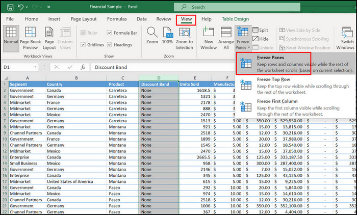
How to Freeze Multiple Panes in Microsoft Excel (Rows & Columns)
Freezing multiple columns and rows in an excel sheet is quite a similar process you read earlier. But, in the earlier section, you learned how to columns and rows (individually). You’ll learn how to lock them in a combined method in this passage.
Here’s the procedure to freeze multiple panes in MS Excel:
- Launch Microsoft Excel and open the sheet you want to modify.
- Select a cell that is last to the row and right to the last column you want to freeze. For example, if you want the first three rows and two columns to be frozen, click on cell C5.
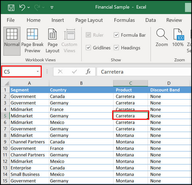
- Follow the same process; go to the view tab > Freeze panes > Freeze panes.
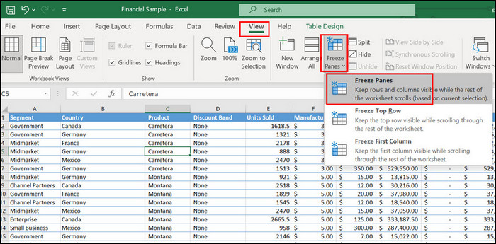
Additional Tips: You can freeze as many panes as you want with this approach. For instance, If you select the E8 cell and freeze panes, rows 1-7 and columns A-D will be frozen.
How to Unfreeze Panes in Microsoft Excel
Unlocking the rows and columns in MS Excel is quite the same process as freezing them. However, if you don’t know the process, follow further steps.
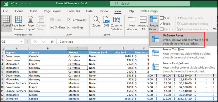
Here are the steps to unfreeze rows and columns in Excel:
- Select all the rows and columns that are locked.
- Go to the view tab > Freeze panes > Unfreeze panes.
You are good to go. If you want to freeze Excel panes in one click, try the following method.
The magic button is the quick access toolbar that you can use to freeze excel panes with a single click. When you have to freeze panes in multiple spreadsheets, you can use this magic button instead of manually locking the panes.
Here are the steps to activate the magic freeze button:
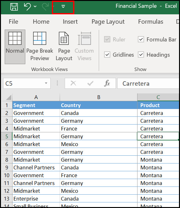
- Launch Microsoft Excel on your computer.
- Click on the down arrow button from the top.
- Select More Commands from the list.
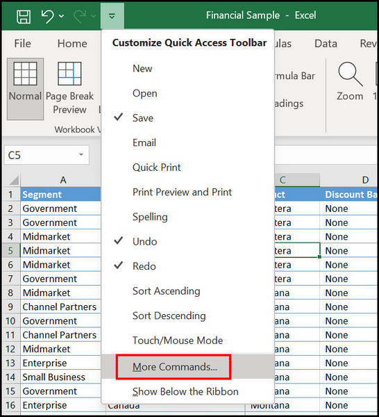
- Click on Quick Access Toolbar from the left pane.
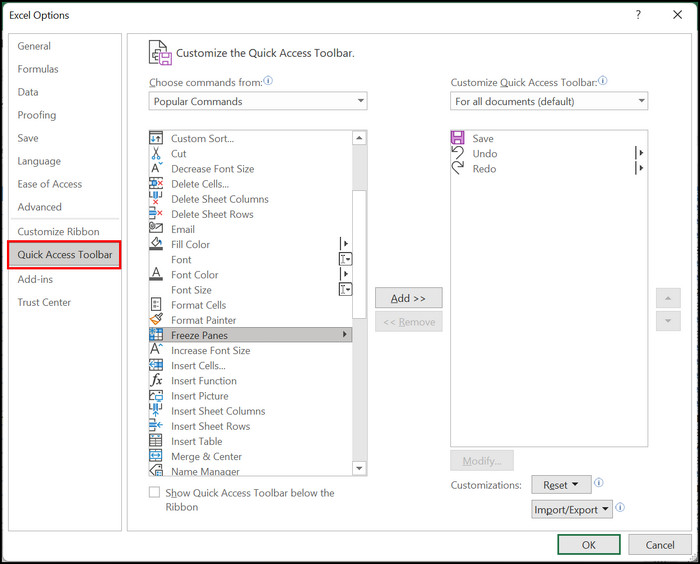
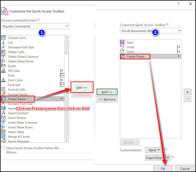
- Locate and click Freeze Panes from the popular commands section.
- Select Add from the middle of the window.
- Click Ok to save the changes.
After you add the magic button, select the rows/columns you want to lock. Click the magic button from the dashboard.
Have further queries regarding freezing the rows and columns? Check out the following section to clear out your confusion.
Frequently Asked Questions
How do I freeze specific panes in Excel?
Select the row below the rows you want to keep visible when you scroll. Click on View > Freeze Panes > Freeze Panes.
How do I freeze the first 3 rows in Excel?
Select row number four in your excel sheet. After that, the process is simple; View tab > Freeze Panes > Freeze Panes.
Can you freeze only certain rows in Excel?
Yes, you can freeze only one row in MS excel. Go to the View tab > Freeze panes > Freeze top row.
Wrapping Up
Throughout this article, I’ve introduced multiple ways of freezing panes in Microsoft Excel. Those will help you to keep the columns/rows visible when you scroll through.
Nevertheless, if any of these methods seem complicated to you, or you have any queries regarding this topic, our comment box is always open.
Just feel free to share your thoughts.