Randomizing lists in Excel is handy if you want to perform various experiments or demonstrations using the application. However, if you are just starting with Excel, you might be unaware of how you can randomize a list in Excel. It’s crucial to understand how to use Excel’s databases and formulae if you work with data or are considering a career involving data. Data analysis with Excel often requires you to randomize a list as well.
As someone with years of experience in Excel, I have randomized plenty of lists while performing different kinds of tasks. In this tutorial, I will share various methods you can use to randomize lists in Excel.
So keep reading this article till the end to learn how to randomize a list in Excel.
Why is Randomization Important in an Experiment in Excel?
In an experiment, randomization refers to assigning values at random. When working on Excel, you may want to create a random list to test a hypothesis.
The results of an experiment will be OK, thanks to randomization, which eliminates bias. For the experiment results to be as precise as possible, it ensures that the groups created for performing the experiment are as similar as possible.
Additionally, it aids in the control of undetected factors that may cause results to deviate from those expected.
The randomly chosen sample is intended to be representative of the population, and because there was no researcher interference, the result was pretty reasonably decided.
Randomizing the experiments can obtain the most accurate cause-and-effect linkages between the variables.
In Excel, randomizing lists can thus eliminate bias, and you can test your hypothesis on randomized values. You can also use the list randomizing feature to distribute tasks more efficiently.
It ensures that all genders, castes, and races are represented in the random selection and that the groupings are not too dissimilar.
Researchers use a randomized approach to control the explanatory variable’s values. Therefore, we can infer a causal relationship between the explanatory and response variables if we observe it.
Related content you should read about how to install Macro in Excel?
What Are the Functions for Randomizing a List in Excel?
There is more than one function available for you to use if you want to randomize a list in Excel. Some of the functions are RAND, RANDBETWEEN, RANDARRAY, etc. I will discuss some of them here so you can understand the arguments well enough.
Here are the functions used to randomize a list:
1. RAND
RAND generates a randomly generated real number higher than or equal to 0 and less than 1 that is dispersed evenly. A new random real number is returned every time the worksheet is calculated.
As of Excel 2010, the Mersenne Twister Algorithm is used to generate random numbers. There are no arguments in the RAND function syntax.
Enter =RAND() in the formula bar and press F9 to switch the formula to a random number if you want to generate a random number using RAND but don’t want the numbers to vary each time the cell is calculated. You will only be left with a value after the formula calculates it.
If you want to increase the upper limit for the generated numbers, use =RAND()*X, with X being the upper limit you want to set.
Use =INT(RAND()*X) to ensure that the generated numbers are integers, which you may know as whole numbers.
Follow our guide to know how to copy values without formulas on Excel?
2. RANDBETWEEN
RANDBETWEEN returns a random integer value within the range of integers you provide. A new random integer number is returned every time the worksheet is calculated.
While RAND generates a random set of real numbers between 0 and 1 unless the upper limit is modified, RANDBETWEEN can only provide you with randomized integer numbers. However, you can set the lower and upper limits as input arguments.
=RANDBETWEEN(lower, upper) is what the syntax of this function looks like when you type it in the formula bar. Instead of lower and upper, use integer values, with the second argument upper being the larger number and the first argument lower being the smaller.
Any calculation that employs the RANDBETWEEN function is updated with a new random number whenever the worksheet is recalculated either manually (hit F9), by inserting a formula or data in a separate cell, or both.
3. RANDARRAY
An array of random numbers is the output of the RANDARRAY function. You can define the minimum and maximum values, the number of rows and columns to fill, and whether to return whole numbers or decimal values.
It is a very flexible and powerful function.
=RANDARRAY([row],[column],[min],[max],[set]) is how the syntax looks like. With all the arguments being optional.
Here are the arguments explained:
- Replace row with the number of rows that you want to be returned.
- Replace column with the number of columns that you want to be returned.
- Replace min with the minimum number that you want to be returned.
- Replace max with the maximum number that you want to be returned.
- Replace set with a logical value. This needs to be either True or False. True will return numbers as integers, and False will return numbers as real numbers.
RANDARRAY will return a single value between 0 and 1 if you do not provide a row or column argument. The default values for RANDARRAY are 0 and 1, respectively, if no minimum or maximum value parameter is provided.
Otherwise, RANDARRAY will produce a #VALUE! Error. The minimum number argument must be smaller than the maximum number. RANDARRY defaults to FALSE or a decimal value if you don’t supply a whole number parameter.
The RAND function does not produce an array, so RAND would need to be copied throughout the entire range. RANDARRAY is different because it does create an array.
Check out the easiest way to fix Microsoft Excel freezing or slow.
How to Randomize a List in Excel?
If you have understood all the functions described in the above section, then you probably already understand how to randomize a list in Excel.
Just to confirm, I will show you an example with each function. Applying a function in a formula and then duplicating that formula in other cells in a column is most of the work that is required. Again, a thorough understanding of the function is required to know what you are doing.
Here are the methods to randomize a list in Excel:
1. Using RAND
You can use the RAND function to generate random real numbers between 0 and 1. But you can modify the formula to change the number type or the upper and low limit.
Using the RAND function, let’s try to generate 10 random integers from 1 to 50.
Follow these steps to generate 10 random integers from 1 to 50 using the RAND function:
- Add a new column next to the list of names you wish to randomize. Skip this step if your dataset just contains a single column.
- Enter the RAND formula into the first cell of the newly added column: =INT(RAND ()*50)
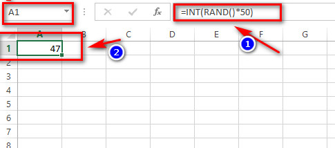
- Duplicate the formula down the column. You can double-click the fill handle to complete this action quickly. For this example, fill the following 9 entries in the column.
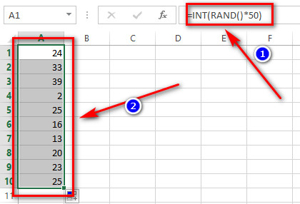
You would get decimal values if you simply used the RAND function without the INT function. The option to get decimal values will not be available for the following function.
Also related to this guide Mail Merge in Outlook with Excel & Word.
2. Using RANDBETWEEN
The RANDBETWEEN function does not generate real numbers. Let’s use this function to generate 10 random integers between 10 and 50.
Follow these steps to generate 10 random integers from 10 to 50 using the RANDBETWEEN function:
- Add a new column next to the list of names you wish to randomize. Skip this step if your dataset just contains a single column.
- Enter the RANDBETWEEN formula into the first cell of the newly added column: =RANDBETWEEN(10,60)
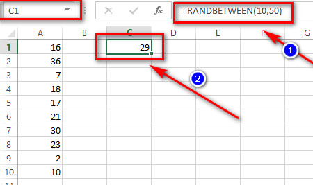
- Duplicate the formula down the column. You can double-click the fill handle to complete this action quickly. For this example, fill the following 9 entries in the column.
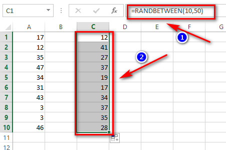
RANDBETWEEN is useful when working with integer values within a fixed range. Move on to the following formula if you want to add more control.
Check out the easiest way how to randomize photos in a folder?
3. Using RANDARRAY
The RANDARRAY function is much more potent than the two previous functions.
You can set what type of number you want to generate and how many you will spawn with a fixed number of rows and columns, with this function’s maximum and a minimum of the generated numbers being settable.
Using this function, let’s try to find 24 random integers from 1 to 100 distributed across 6 rows and 4 columns.
Follow these steps to generate 24 random integers from 1 to 100 distributed across 6 rows and 4 columns using the RANDARRAY function:
- Add a new column next to the list of names you wish to randomize. Skip this step if your dataset just contains a single column.
- Enter the RANDARRAY formula into the first cell of the newly added column: =RANDARRAY(6,4,1,100,TRUE)
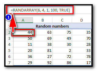
You can combine this function with others to do more amazing things in Excel. This function is only available from Excel 2019 onwards.
FAQs
How to sort a randomized list in Excel?
The values in a related range are used to sort a range using the SORTBY function. The SORT function always sorts in ascending order. Look up the function names to learn more.
How to index a randomized list in Excel?
You can index a randomized list in Excel using the INDEX function. The INDEX function returns a value or a reference to a value from within a table or range. Look up the function name to learn more.
How to sort an already generated randomized list in Excel?
Click Sort & Filter > Sort Smallest to Largest under the Home tab. If you like, you may instead select Sort Largest to Smallest.
Conclusion
You can use the RAND, RANDBETWEEN, and RANDARRAY functions in Microsoft Excel to reorder items in a list in random order. The functions generate random numbers that you can use to select things from your list randomly.
Use RANDARRAY if you have the function in your version of Excel. It offers you a lot of flexibility regarding the list being generated.
If you have any further queries, please comment below!
